Presentation of the complementary filter

Let two sensors \(X\) and \(Y\) giving measurements \(x\) and \(y\) on the same quantity \(q\).

\(X\) is assumed to have a drift free noise model, which means the average of the noise over some period of time is zero. This is the case for zero-mean gaussian noise. However it has a lot of jitter, or high frequency noise, and potentially updates less frequently than \(Y\).

\(Y\) is assumed to have a drifting noise model, which means there is an error changing over long periods of time. This could result from random march in integrated sensor measurements like rotation estimation from a sole gyroscope. However its high frequency noise is very small compared to that of \(X\).

The complementary filter uses the idea that a signal can be decomposed as a low-frequency and a high-frequency components:
\[x = x_{low frequency} + x_{high frequency}\] \[y = y_{low frequency} + y_{high frequency}\]
And if the cutoff frequency is the same for both signals, is becomes possible to exchange them. The complementary filter would thus estimate \(q\) by replacing the drifting low-frequency component of \({y}\) by the non-drifting low-frequency component \({x}\), while the less jittery high frequency of sensor \(Y\) is kept:
\[\hat{q} = x_{low frequency} + y_{high frequency}\]
We denote the low frequency components as \(\bar{x}\) and \(\bar{y}\). The same low-pass filter of smoothing parameter \(\alpha\) is applied to both signals:
\[\bar{x}^{n+1} = \alpha(\bar{x}^{n}) + (1-\alpha)(x^{n+1}) \] \[\bar{y}^{n+1} = \alpha(\bar{y}^{n}) + (1-\alpha)(y^{n+1}) \]
And the state estimate \(\hat{q}\) is obtained with
\[\hat{q}^{n} = y^n + (\bar{x}^{n} - \bar{y}^{n})\]

Basic complementary filter example

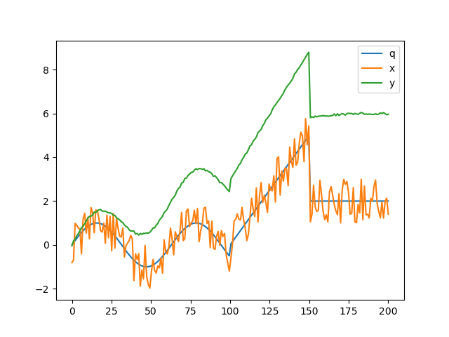
Values are simulated with the following noise models:
\[x^n = q + G(1, 0) \] \[y^n = q + G(0.05, 0) + 4\sin(n/120) \]
The measurements \(x\) and \(y\) and the ground truth \(q\) are plotted below:


When the complementary filter is applied, as \(\alpha\) gets larger an offset between the ground truth and the estimate appears:


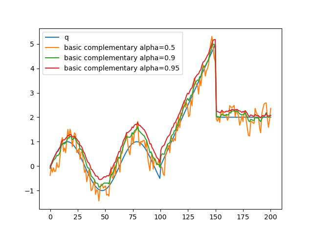
This is due to the fact that the filter is applied at the end of the low-pass filtering window. The average only takes into account the values before instant \(n\) so it is biased and doesn't account for the fact that the drift of \(Y\) grows with \(n\). Even worse, that drift is not a linear function of n, so the rate of change is not constant over time.

Introducing derivatives in the state estimate

Taking inspiration from the state estimates used with kalman filtering, it is possible to modify \(x\) and \(y\) into \(\mathbf{x}\) and \(\mathbf{y}\) :
\[\mathbf{x} = (x, \frac{dx}{dn}, \frac{d²x}{dn²}, ... ) \]
Getting derivatives is complicated with the low-pass filter we used, but it is possible to get the difference between the average and the current value at each \(n\):
\[\Delta x^n = x^n - \bar{x}^n \] \[\Delta² x^n = \Delta x^n - \bar{\Delta x}^n \] \[...\]
Which is are measures of the growth of \(x\) in the latency window of the filter, abstracting the notion of time. The state estimate becomes:
\[\mathbf{x} = (x, \Delta x, \Delta² x, ... ) \]
And the final estimate of \(q\):
\[\hat{q}^{n} = y^n + (\bar{x}^{n} - \bar{y}^{n}) + (\bar{\Delta x}^{n} - \bar{\Delta y}^{n}) + (\bar{\Delta² x}^{n} - \bar{\Delta² y}^{n}) + ...\]

Simulation at order 1

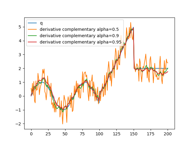
The estimate sticks more with the tendency of sensor \(X\).

Simulation at order 2

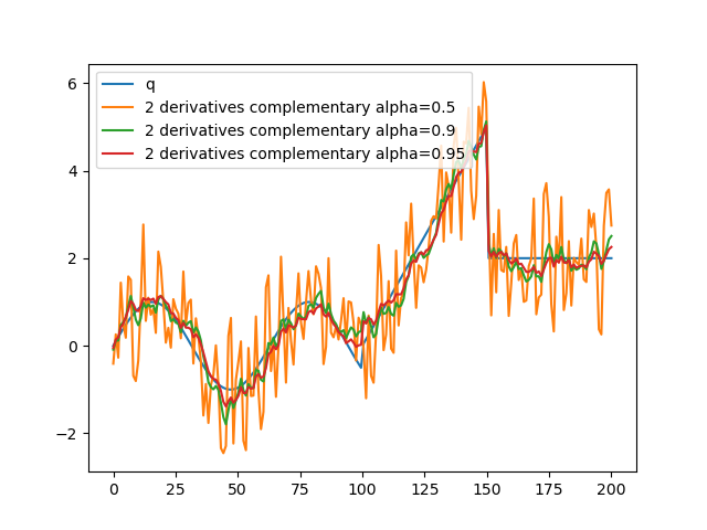
The estimate becomes disturbed by small scale variations in \(x\).

So like when designing Kalman filters, estimating derivatives too far can reduce the performances of the filter.